|
Week five has come and gone and we are officially over halfway through the REU. I’m convinced time is thinner on the Oregon coast because it’s so easy to slip through three days and not even realize it until you’ve checked your calendar. This week brought some unexpected twists and turns. First of all, I finished my kelp density estimates for all fifteen videos and created a couple figures to model my results. At the first two sites in Haida Gwaii there were a range of 1.3-1.5 kelp stipes per square meter. At the third site there were closer to 2 stipes per square meter. And there were 0 stipes at the final two sites. Zero as in, I watched all four videos the prescribed three times and not a single stipe appeared in frame the entire time. I wasn’t sure what to make of this result but Dr. Galloway seemed excited by this revelation! Speaking of Dr. Galloway, he very generously offered to let me help with a project in the lab this week. He needed to collect some data on the calories present in red sea urchin gonads (reproductive organs) and set about doing so mid-week. With the help of another grad student, we created a makeshift assembly line in which I would record the dimensions of each whole urchin, Dr. Galloway would crack the urchin open and dissect out a gonad, I would record the wet mass of the gonad, and then a sample of a different gonad would be stored for testing. 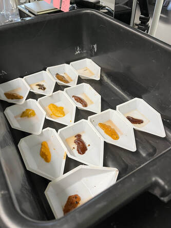 Urchin gonads before the drying oven. We harvested thirteen gonads in total and put them in the drying oven for 48 hours before I went back to collect them and record the dry mass of the gonads. The alternate samples were put in a freeze dryer and then ground up and compacted into pellets to use for analysis in the bomb calorimeter. A bomb calorimeter is, in a word, sorcery. Well no, it’s actually an instrument in which you can put a dry sample of some substance into a metal capsule (the bomb), pressurize the capsule with 100% oxygen, combust the sample until it is entirely consumed, and then derive how many calories the sample contained from the energy released by the combustion. Also, they don’t tell you this in the manual, but you can only use the calorimeter during a full moon, you have to sacrifice a lock of your hair into the bomb, and you have to perform some sort of pagan-sounding chant before you turn it on or else it won’t work. 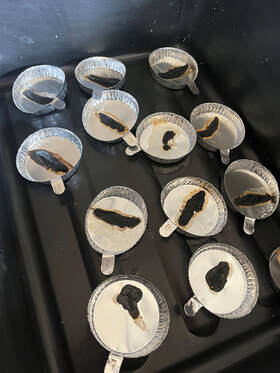 Urchin gonads after the drying oven. Anyway, the urchin project was both an extremely fun and informative side-quest this week and I’m so glad I was able to participate! I think I’ll spend the next week planning my poster and working on a new set of kelp videos. See you then!
0 Comments
Welcome to week four! As I’m writing this my hair is still wet from the shower I took after a long morning of tide-pooling. We left for Qochyax Island at seven fifteen this morning because that’s when the tide was lowest. During a low tide you can scramble down the cliffside along Sunset Bay and walk to the island, although it’s important to keep an eye on the time because if you leave too late the tide will have returned and you’ll be swimming back. We saw several cool creatures including the tiniest little nudibranch (I’m forgetting which species, my apologies) and more purple urchins than I knew how to comprehend. 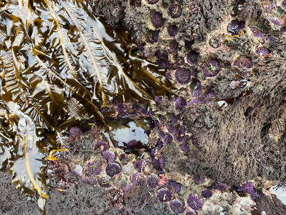 A bed of purple urchins. On the academic front, I submitted my proposal this Tuesday and began to work on my proposal presentation for next Tuesday. I’m so excited to hear what everyone has been working on these last few weeks in their respective labs. I also finished pulling stills from the Haida Gwaii videos and formatting the file names for every screenshot into my excel spreadsheet, which is now 271 cells long. I think I’m beginning to earn the “Microsoft Excel” qualification on my resume. I then calculated the mean widths for each set of stills and the standard deviation between each width measurement. After speaking with Dr. Galloway we’ve decided that a quick way to get a sense of how significant the difference between the width mean for 10 stills versus 20 stills is a two sample t-test. This means that after conducting the test, which compares the mean of two data sets, if the resulting value is greater than 0.05 then there is no significant statistical difference between each mean, and possibly, no reason to collect 20 stills versus 10. However, if the t-test value is below 0.05, there IS a significant difference between each mean and I might wonder if I need to collect even more stills to paint an accurate picture of the contents of each video. 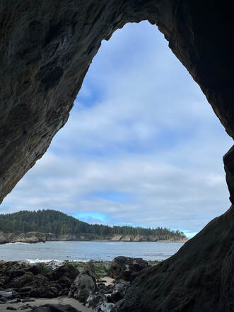 Sunset Bay from inside a cave. So far my results have been well over the 0.05 threshold, ranging from 0.5-0.7, so it seems like if nothing else my data is consistent! Could be consistent and wrong, but consistent nonetheless! In addition, I counted the visible kelp in each video three separate times and began doing the density calculations (kelp abundance/area in m2). I’m still working out how many significant digits I want to include in my final density-estimates so I’ll share some more results next week. Finally, and possibly most importantly, it’s time for a round rock update!!! [pause for applause, cheering, excited utterances etc.] On Wednesday after Ytxzae and I finished a run we decided to wander down to the OIMB beach during low tide and lo’ and behold, nestled in the rocks where we left it behind last time was The round rock. We still have not decided what to do with it but after several more people suggested that we break it open in hopes of finding a highly unlikely geode or try leaving it in water overnight to see if it disintegrates, the rock has been relocated to the floor of my dorm room for the time being. It is quite an effective door stopper I must say. 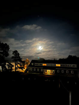 OIMB campus at night with a full moon. That’s about all I can think of to update this week but there are plenty more exciting things to come. Talk to you then!
What to say about week three. I suppose I’ll start at the beginning. Monday was the fourth of July and we had a delicious picnic on campus with all the interns and UO students and some of the mentors and professors. I ate a few of the freshest oysters I’ve ever had given that they were harvested from the ocean across the street (have I mentioned how much I love having an ocean across the street?) and played some friendly volleyball with the other interns. I only hit the ball into the creek once and it was hot enough that it dried almost instantly. The rest of the afternoon I spent swimming with Ytxzae and hanging out on the jetty with Flynn and it was all very pleasant and relaxing. 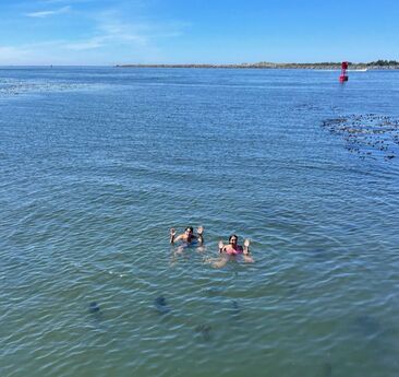 I spent most of the work week prodding at my methodology and praying there were no design flaws. Some of the details I mulled over were: how the depth of the diver’s position affects the size of the scale, if pulling stills every fifteen seconds provides enough data to resist the skew of outliers, and how to ensure I’m only counting kelp within the approximated rectangle of the diver’s course. First, I decided to write-off the depth of the footage off-bottom as a random effect of my model because I’m only going for a flat-bottom estimate, meaning the survey is 2-D. The height of the diver's vantage point should not matter because the size of the laser scale adjusts proportional to its distance from the sea floor. Second, I’ve decided to calculate the width means and standard deviations for the original ten stills AND for an expanded data set of twenty stills per video, in order to compare the values and assess both precision (the similarity of the values to each other) and accuracy (the difference between the experimental widths and the actual width of the transect). Precise values would look like: 1.2, 1.3, 1.2, 1.1, 1.2, while an accurate value would be 1.2 if the true width of the transect was also 1.2. And finally, since I am manually collecting still images I have some agency in where/when I take a screenshot. I’ve decided that I’ll only capture a still when the diver is looking straight ahead and not at a random point off to the side, to prevent collecting a width that does not fall within the sample boundary. 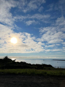 Have a look at this nice view while you take your deep breath. I just took a very long and deep breath after typing all of that out, please feel free to take a deep breath with me as you have just read everything I typed out. Many thanks.
Well, I’ve embarked on some revisions to my project so I think I’ll spend the next week doing a little more cleanup and hopefully start sharing some results! With the arrival of Week Two I am feeling simultaneously excited and uncertain. On Monday I spent much of my time watching and rewatching a batch of thirty videos collected from Dr. Galloway and his team’s diving trip to Haida Gwaii in 2021. Each video belongs to one of three transects. The first transect spans between the shore and a depth of 10 meters, the second extends to a depth of 20 meters, and the third reaches 30 meters deep. A diver covers 30 meters (in length) of footage per video from two vantage points. The first is a benthic perspective that captures the seafloor along the transect and the second is a pelagic view facing upward toward the surface. Ultimately, these videos and our investigation into underwater video surveying aim to pin down some standard practices for monitoring the health and species composition of kelp forests. Bull kelp (Nereocystis luetkeana) in Pacific Northwest kelp ecosystems have declined by nearly 90 percent since 2014 for a myriad of reasons. These include Marine Heat Waves (MHW’s), which disrupt the distribution of nutrients along the coast, and Sea Star Wasting Disease, which wiped out the majority of sea urchins’ natural predators and in turn facilitated the formation of urchin barrens. For the restoration of bull kelp to transpire we need to develop viable methods of monitoring the status of the ecosystem to oversee the process. 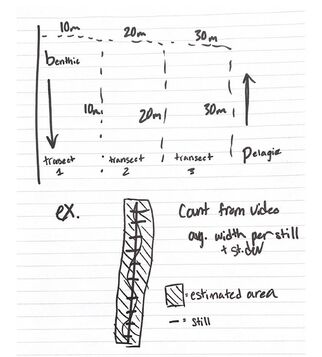 An attempt at a diagram of the video content described above. This is where my individual research slots in. I will attempt to calculate a flat-bottom density estimate of bull kelp present in the Haida Gwaii videos. The methodology is fairly simple. For each video I will pull a still image every fifteen seconds, this works out to about ten stills per video. For each still I will digitally create an 11 centimeter scale helpfully provided by two lasers projected from the diver onto the seafloor and kept constant for the duration of the dive footage. I will use the scale to measure the width of the visible transect and then average the widths I collect from all ten stills. Using the 30 meter transect length and the approximated width to find the area of the transect, all that’s left to do is count the bull kelp from the same video and determine how many bull kelp are present per square meter! So basically when I swore I would never use geometry or statistics in “real life” it was a blatant lie. Suddenly standard deviations are an uncomfortably common occurrence in my day-to-day. 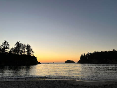 The beach at sunset. On the social side of things, last weekend we took an REU camping trip to Sunset Bay State Park. I learned several important life lessons: 1. You can make an incredibly successful s’more with a Crunch bar or Butterfinger, 2. Crows are capable of being extremely loud especially when they band together and chorus at five AM. I understand why a group of them is called a “murder” now, they genuinely sounded like they were committing a felony, 3. The sunsets in Oregon are gorgeous when you watch them from the shore, 4. The Pacific Ocean is so cold. I already knew that but reiterating it gives me validation.
Overall, I had another spectacular week at OIMB and I’m excited to start working on my proposal this weekend to hopefully kickstart another! |
AuthorHello! My name is Catalina, welcome to my blog! I am a rising Junior at NYU pursuing a degree in Biology and I'm from Sunnyvale, California. This summer I am working in Dr. Aaron Galloway's Coastal Trophic Ecology (CTE) lab developing video survey methodology applied to kelp forest monitoring. Thanks for reading! Archives
August 2022
Categories |
 RSS Feed