|
With the arrival of Week Two I am feeling simultaneously excited and uncertain. On Monday I spent much of my time watching and rewatching a batch of thirty videos collected from Dr. Galloway and his team’s diving trip to Haida Gwaii in 2021. Each video belongs to one of three transects. The first transect spans between the shore and a depth of 10 meters, the second extends to a depth of 20 meters, and the third reaches 30 meters deep. A diver covers 30 meters (in length) of footage per video from two vantage points. The first is a benthic perspective that captures the seafloor along the transect and the second is a pelagic view facing upward toward the surface. Ultimately, these videos and our investigation into underwater video surveying aim to pin down some standard practices for monitoring the health and species composition of kelp forests. Bull kelp (Nereocystis luetkeana) in Pacific Northwest kelp ecosystems have declined by nearly 90 percent since 2014 for a myriad of reasons. These include Marine Heat Waves (MHW’s), which disrupt the distribution of nutrients along the coast, and Sea Star Wasting Disease, which wiped out the majority of sea urchins’ natural predators and in turn facilitated the formation of urchin barrens. For the restoration of bull kelp to transpire we need to develop viable methods of monitoring the status of the ecosystem to oversee the process. 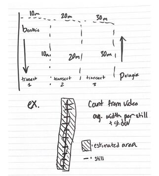 An attempt at a diagram of the video content described above. This is where my individual research slots in. I will attempt to calculate a flat-bottom density estimate of bull kelp present in the Haida Gwaii videos. The methodology is fairly simple. For each video I will pull a still image every fifteen seconds, this works out to about ten stills per video. For each still I will digitally create an 11 centimeter scale helpfully provided by two lasers projected from the diver onto the seafloor and kept constant for the duration of the dive footage. I will use the scale to measure the width of the visible transect and then average the widths I collect from all ten stills. Using the 30 meter transect length and the approximated width to find the area of the transect, all that’s left to do is count the bull kelp from the same video and determine how many bull kelp are present per square meter! So basically when I swore I would never use geometry or statistics in “real life” it was a blatant lie. Suddenly standard deviations are an uncomfortably common occurrence in my day-to-day. 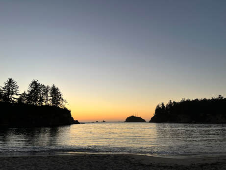 The beach at sunset. On the social side of things, last weekend we took an REU camping trip to Sunset Bay State Park. I learned several important life lessons: 1. You can make an incredibly successful s’more with a Crunch bar or Butterfinger, 2. Crows are capable of being extremely loud especially when they band together and chorus at five AM. I understand why a group of them is called a “murder” now, they genuinely sounded like they were committing a felony, 3. The sunsets in Oregon are gorgeous when you watch them from the shore, 4. The Pacific Ocean is so cold. I already knew that but reiterating it gives me validation.
Overall, I had another spectacular week at OIMB and I’m excited to start working on my proposal this weekend to hopefully kickstart another!
1 Comment
Barb Fritschen
7/7/2022 03:53:36 pm
Throughly enjoying your posts, Cat! And you are making my math teacher’s heart proud!😍 Leave a Reply. |
AuthorHello! My name is Catalina, welcome to my blog! I am a rising Junior at NYU pursuing a degree in Biology and I'm from Sunnyvale, California. This summer I am working in Dr. Aaron Galloway's Coastal Trophic Ecology (CTE) lab developing video survey methodology applied to kelp forest monitoring. Thanks for reading! Archives
August 2022
Categories |
 RSS Feed